
CMP3751M Machine Learning
Data Mining Algorithms代写 Data import, summary, preprocessing and visualization Selecting an algorithm Algorithm Design Model Selection

Algorithms for Data Mining
Section 1: Data import, summary, preprocessing and visualization
Importing Data
The nuclear power plant data set is available in CSV format, which means that each value is separated by a comma, the feature header is defined on the first line, and then the data.Data Mining Algorithms代写
| Status |
| Power_range_sensor_1 |
| Power_range_sensor_2 |
| Power_range_sensor_3 |
| Power_range_sensor_4 |
| Pressure_sensor_1 |
| Pressure_sensor_2 |
| Pressure_sensor_3 |
| Pressure_sensor_4 |
| Temperature_sensor_1 |
| Temperature_sensor_2 |
| Temperature_sensor_3 |
| Temperature_sensor_4 |
By storing the data set in a data frame, can easily perform mathematical operations such as calculating the mean, standard deviation, minimum, and maximum.Data Mining Algorithms代写
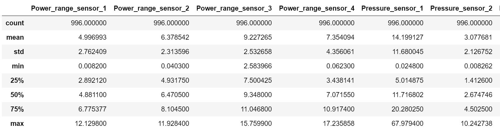
Data summary
There are 13 features in total: 4 sensors for each reading type, including power range, pressure and temperature. The last feature contains categorical variables representing the state of the reactor, either “normal” or “abnormal”. There are no missing or null values in the data set.Data Mining Algorithms代写
———————————————————————————————————————-
Data  Assignment2-dataset-nuclear_plants.csv

Features count:13

Records count:996


Feature   Mean

Power_range_sensor_1      4.996993

Power_range_sensor_2      6.378542

Power_range_sensor_3      9.227265

Power_range_sensor_4      7.354094

Pressure _sensor_1       14.199127

Pressure _sensor_2        3.077681

Pressure _sensor_3        5.748279

Pressure _sensor_4        4.997002

Temperature_sensor_1      8.155479

Temperature_sensor_2     10.001593

Temperature_sensor_3     15.186910

Temperature_sensor_4      9.933125

dtype: float64
Pressure_sensor_1 is much larger than other pressure averages, and temperature_sensor_3 is also larger than other temperature values. This may indicate that there may be outliers in the data. However, this difference may be reasonable, as each sensor reads at a different location within the reactor.Data Mining Algorithms代写
Feature   Std Dev

Power_range_sensor_1      2.762409

Power_range_sensor_2      2.313596

Power_range_sensor_3      2.532658

Power_range_sensor_4      4.356061

Pressure _sensor_1       11.680045

Pressure _sensor_2        2.126752

Pressure _sensor_3        2.526864

Pressure _sensor_4        4.165490

Temperature_sensor_1      6.174639

Temperature_sensor_2      7.336233

Temperature_sensor_3     12.159565

Temperature_sensor_4      7.282817

dtype: float64
The standard deviation of the pressure sensor 1 and the temperature sensor 3 is much larger than other sensors. This may indicate outliers in the data, but may be the result of different sensor positions.Data Mining Algorithms代写
Feature                        Min

Power_range_sensor_1     0.008200

Power_range_sensor_2     0.040300

Power_range_sensor_3     2.583966

Power_range_sensor_4     0.062300

Pressure _sensor_1       0.024800

Pressure _sensor_2       0.008262

Pressure _sensor_3       0.001224

Pressure _sensor_4       0.005800

Temperature_sensor_1     0.000000

Temperature_sensor_2     0.018500

Temperature_sensor_3     0.064600

Temperature_sensor_4     0.009200

dtype: float64


Feature                       Max

Power_range_sensor_1     12.129800

Power_range_sensor_2     11.928400

Power_range_sensor_3     15.759900

Power_range_sensor_4     17.235858

Pressure _sensor_1       67.979400

Pressure _sensor_2       10.242738

Pressure _sensor_3       12.647500

Pressure _sensor_4       16.555620

Temperature_sensor_1     36.186438

Temperature_sensor_2     34.867600

Temperature_sensor_3     53.238400

Temperature_sensor_4     43.231400

dtype: float64
The max-min value of each function shows the highest data point read by each sensor. The maximum value of pressure sensor 1 is much higher than other pressure sensors, which again indicates that there may be abnormal values in the data.Data Mining Algorithms代写
———————————————————————————————————————-
Visualization
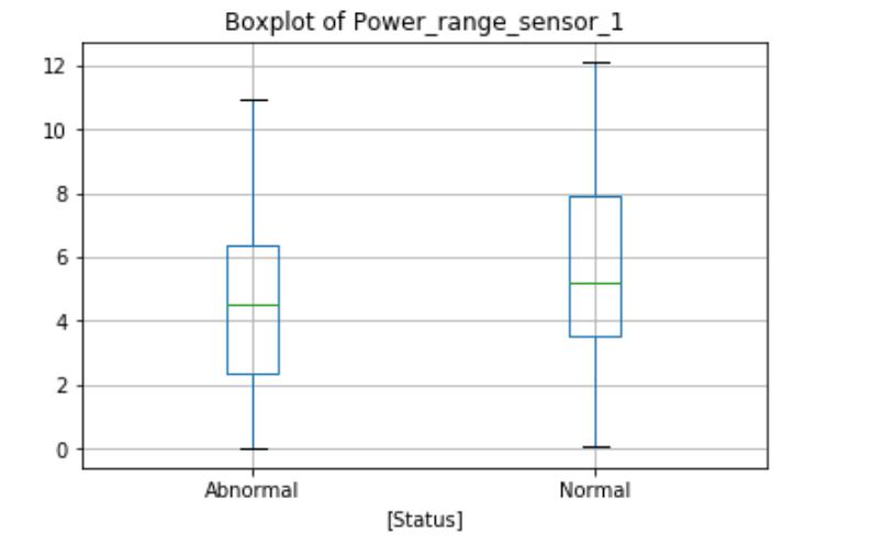
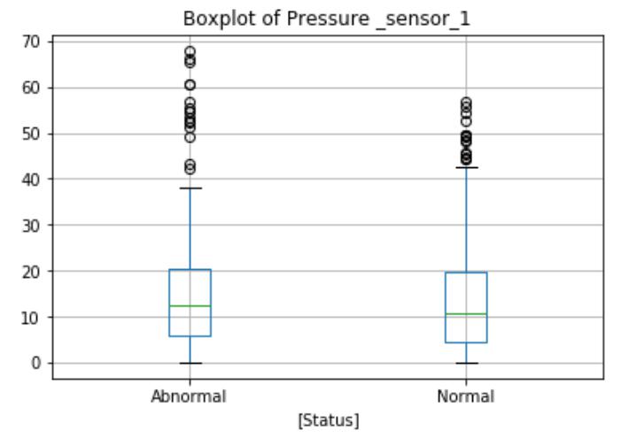
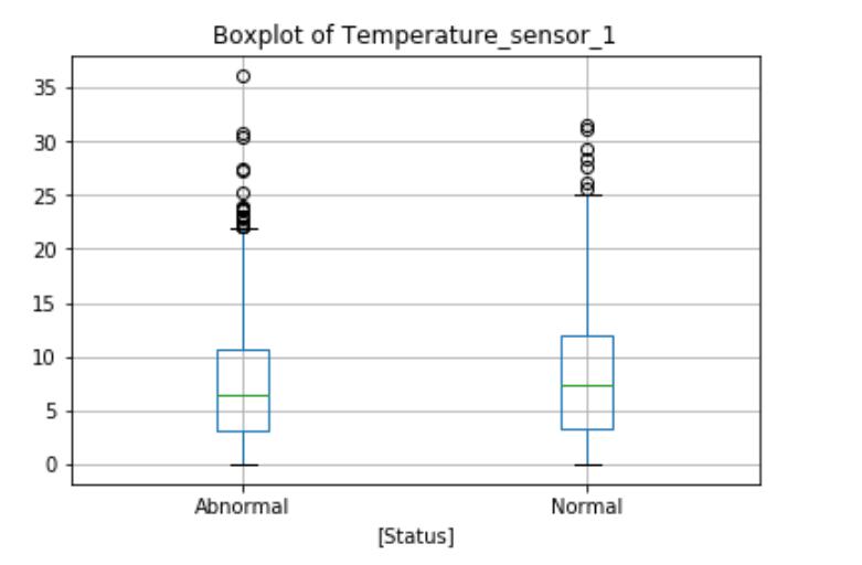
The Power_range_sensor_1 boxplot shows the differences in the normal and abnormal state categories. during normal operation, the average reactor power is slightly higher, and the maximum value and interquartile range are also higher. The boxplot will identify outliers above or below the maximum indicator for the circle, as shown here, there are no obvious outliers in this function. But the Temperature_sensor_1 and Pressure _sensor_1 boxplots show outliers exist in both data categories. These extremes may be measurement errors or natural outliers, which means that they are not errors but novelty in the data.Data Mining Algorithms代写
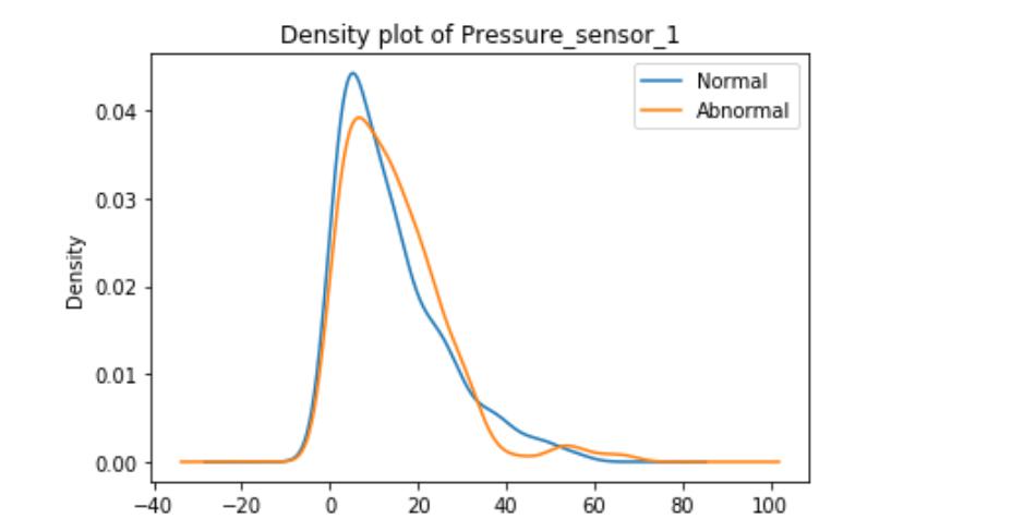
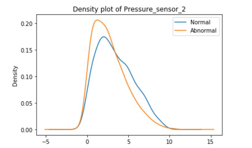
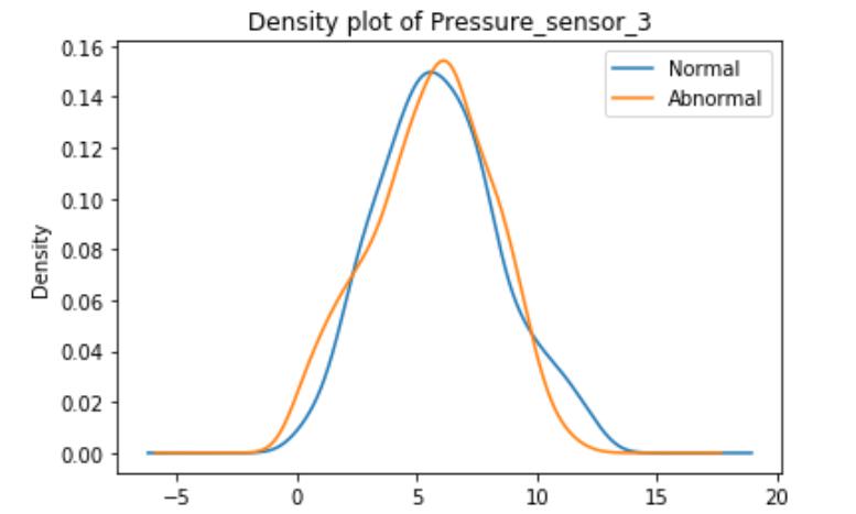
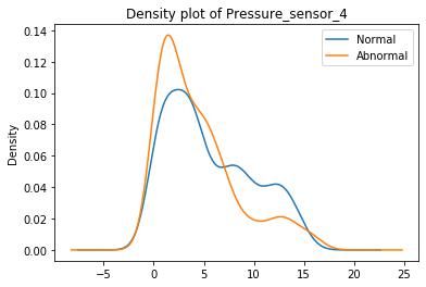
These graphs are density plots of the feature Pressure_sensor. The density plot visualizes the distribution of data through the continuous sensor values.
As suggested, there may be some underlying error or unexplained novelties within the data.Data Mining Algorithms代写
Preprocessing data
The data provided includes data from 3 different scales. Power, pressure and temperature are all measured using different indicators. Due to the deviation of one element from another in the network, differences in scale may lead to differences within the model. Therefore, before using the data in the ANN, the data must be normalized or standardized so that all functions reach the same scale.Data Mining Algorithms代写
Data standardization and standardization use the StandardScaler model and the standardized model in the Sklearn preprocessing sub-library.Data Mining Algorithms代写
They refer to the process of rescaling numeric attributes to the range of 0 and 1.
#--------Data Standardisation normalisation ---------------------


X = Data.drop("Status", axis=1)


scaler = StandardScaler()

X = scaler.fit_transform(X)

X = preprocessing.normalize(X, norm='l2')
Section 2: Selecting an algorithm
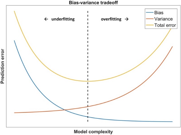
When designing a model, we often hope that the machine can learn a model with small empirical and generalization errors and which performs very well on both the training and test sets, but this is not the case in reality. When the model complexity is higher, the degree of fit to the training set is higher, but the generalization ability of the new sample is reduced, and overfitting (overfitting) occurs at this time.Data Mining Algorithms代写
In order to get a relatively stable model with good generalization ability, we should choose a model with appropriate complexity and good fit.
The complexity of the model gradually increases as the training of the sample progresses. At this time, the error on the training data set will gradually decrease. When the complexity of the model reaches a certain level, the error on the test set will increase with the complexity of the model Increase. It can be seen from the figure that the abscissa value of the red point is the model complexity we expect, and it performs well on both the training set and the test set.Data Mining Algorithms代写
In machine learning, all data is usually divided into three parts: training data set, validation data set, and test data set. Their functions are
Training dataset: used to build machine learning models
Validation dataset: assists in constructing the model, used to evaluate the model during the construction process, to provide an unbiased estimate for the model, and then to adjust the model’s hyperparameter
Test dataset: used to evaluate the performance of the trained final model
Constant use of test and validation sets will gradually make them ineffective. That is, the more times the same data is used to determine the hyperparameter settings or other model improvements, the lower the confidence that these results can be truly generalized to new data that has not been seen before. Note that the validation set usually fails more slowly than the test set. If possible, it is recommended to collect more data to “refresh” the test and validation sets. Restarting is a good way to reset.Data Mining Algorithms代写
Kuhn and Johnson point out in the “Data Splitting Recommendations” that using separate “test sets” (or validation sets) has certain limitations, including:
- The test set is a single evaluation of the model and cannot fully show the uncertainty of the evaluation results.
- Dividing a large test set into test and validation sets increases the bias of model performance evaluation.
- The segmented test set sample size is too small.
- The model may require every possible data point to determine the model value.
- Different test sets generate different results, which results in great uncertainty in the test set.
- The resampling method can make a more reasonable prediction of the performance of the model on future samples.
Therefore, in practical applications, a K-fold cross-validation method can be selected to evaluate the model, which has low deviation and small changes in performance evaluation.
The K-fold cross validation method divides the data set into k mutually exclusive subsets of similar size, and tries to ensure the consistency of the data distribution of each subset. In this way, you can obtain k training-test sets for k trainings and tests.Data Mining Algorithms代写
k usually takes the value 10, which is called 10-fold cross validation. Other commonly used k values are 5, 20, and so on.
Section 3: Algorithm Design
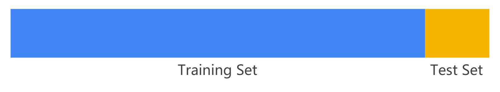
Splitting data
Data is split into a training set and a test set.Data Mining Algorithms代写
- training set—a subset to train a model.
- test set—a subset to test the trained model.
Ensure that the test set meets the following two conditions:
Large enough to produce statistically significant results.
Represents the entire data set. In other words, don’t choose a test set with different characteristics than the training set.
The train_test_split function is imported from the sklearn.model_selection sublibrary. test_size = 0.1 defines the size of the test set as 10% of the total dataset.
Model training
Multilayer Perceptron (MLP) is also called Artificial Neural Network (ANN). In addition to the input and output layers, it can have multiple hidden layers. The simplest MLP contains only one hidden layer, that is, three layers. The structure is as follows:
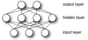
As can be seen from the above figure, the multilayer perceptron layers are fully connected to each other (fully connected means that any neuron in the previous layer is connected to all neurons in the next layer). The bottom layer of a multilayer perceptron is the input layer, the middle is the hidden layer, and the last is the output layer.Data Mining Algorithms代写
To implement a multilayer perceptron classifier, use the MLPClassifier function in the sklearn.neural_network sub-library. This function creates a MLP algorithm model using backpropagation to reduce errors and generate a model that represents the input data. The function takes a number of parameters, including hidden_layer_sizes which defines the number of hidden layers and nodes in each layer.Data Mining Algorithms代写
After defining the model, you can fit it to the training data.
Random forest classifier
In view of the shortcomings of decision trees that are easy to overfit, random forest uses a voting mechanism of multiple decision trees to improve the decision tree. We assume that random forest uses m decision trees. For a tree, it is obviously not desirable to train m decision trees with full samples. Full sample training ignores the law of local samples, which is harmful to the generalization ability of the model. The method of generating n samples uses Bootstrapping method. This is a sampling method with replacement, which produces n samples, and the final result is obtained using the Bagging strategy, that is, the majority voting mechanism.Data Mining Algorithms代写
To implement the random forest classifier, the RandomForestClassifier model function is imported from the sklearn.ensemble sub-library. n_estimators defines the number of trees in the forest, and min_samples_leaf defines the minimum number of samples required at the leaf nodes.Data Mining Algorithms代写
After defining the model, you can fit it to the training data.
result
| MLP Accuracy Score: 0.93 |
| Report: precision recall f1-score support |
| Abnormal 0.96 0.91 0.94 58 |
| Normal 0.89 0.95 0.92 42 |
| accuracy 0.93 100 |
| macro avg 0.93 0.93 0.93 100 |
| weighted avg 0.93 0.93 0.93 100 |
| Tree Accuracy Score : 0.96 |
| Report: precision recall f1-score support |
| Abnormal 0.97 0.97 0.97 58 |
| Normal 0.95 0.95 0.95 42 |
| accuracy 0.96 100 |
| macro avg 0.96 0.96 0.96 100 |
| weighted avg 0.96 0.96 0.96 100 |
This table shows the results of the test set accuracy results.
Section 4: Model Selection
K-fold cross validation: sklearn.model_selection.KFold (n_splits = 10, shuffle = False, random_state = None)
Idea: Divide the training / test data set into n_splits mutually exclusive subsets, use one of them as the validation set at a time, and use the remaining n_splits-1 as the training set. Perform n_splits training and testing to get n_splits.
———————————————————————————————————————-
model_MLP = MLPClassifier()

parameters = {'hidden_layer_sizes':[25,100,500]}

gridsearch = GridSearchCV(model_MLP, parameters, cv=10, iid=False, return_train_score=True)

gridsearch.fit(x_train,y_train)

print(gridsearch.cv_results_['mean_test_score'])

print(gridsearch.best_estimator_)


[0.80475861 0.85952957 0.8929647 ]

MLPClassifier(activation='relu', alpha=0.0001, batch_size='auto', beta_1=0.9,

              beta_2=0.999, early_stopping=False, epsilon=1e-08,

              hidden_layer_sizes=500, learning_rate='constant',

              learning_rate_init=0.001, max_iter=200, momentum=0.9,

              n_iter_no_change=10, nesterovs_momentum=True, power_t=0.5,

              random_state=None, shuffle=True, solver='adam', tol=0.0001,

              validation_fraction=0.1, verbose=False, warm_start=False)


model_RF = RandomForestClassifier()

parameters = {'n_estimators':[10,50,100]}

gridsearch = GridSearchCV(model_RF, parameters, cv=10, iid=False, return_train_score=True)

gridsearch.fit(x_train,y_train)

print(gridsearch.cv_results_['mean_test_score'])

print(gridsearch.best_estimator_)


[0.89835961 0.91746018 0.91965826]

RandomForestClassifier(bootstrap=True, class_weight=None, criterion='gini',

                       max_depth=None, max_features='auto', max_leaf_nodes=None,

                       min_impurity_decrease=0.0, min_impurity_split=None,

                       min_samples_leaf=1, min_samples_split=2,

                       min_weight_fraction_leaf=0.0, n_estimators=100,

                       n_jobs=None, oob_score=False, random_state=None,

                       verbose=0, warm_start=False)

----------------------------------------------------------------------------------------------------------------------
Conclusion
After training a supervised learning algorithm in the form of a multilayer perceptron and a random forest classifier, the random forest model performs more robust and excellent.
Neural networks often require large numbers, and random forest models on small data sets have obvious advantages. Neural networks often require more demanding data preparation, and random forest models generally do not require data processing. And the difficulty of tuning the random forest model is much lower than the neural network. And the interpretation of integrated tree models is generally higher.Data Mining Algorithms代写
Generally speaking, with a small amount of data and many features, integrated tree models are often better than neural networks.
References
Gardner M W, Dorling S R. Artificial neural networks (the multilayer perceptron)—a review of applications in the atmospheric sciences[J]. Atmospheric environment, 1998, 32(14-15): 2627-2636.
Pal M. Random forest classifier for remote sensing classification[J]. International Journal of Remote Sensing, 2005, 26(1): 217-222.
Kriegel H P, Kröger P, Zimek A. Outlier detection techniques[J]. Tutorial at KDD, 2010, 10.
Kohavi R. A study of cross-validation and bootstrap for accuracy estimation and model selection[C]//Ijcai. 1995, 14(2): 1137-1145.
Claeskens G, Hjort N L. Model selection and model averaging[R]. Cambridge University Press, 2008.
Anderson D, Burnham K. Model selection and multi-model inference[J]. Second. NY: Springer-Verlag, 2004, 63.
更多其他:文学论文代写 商科论文代写 艺术论文代写 人文代写 Case study代写 心理学论文代写 哲学论文代写 计算机论文代写


您必须登录才能发表评论。