Normal Probability Density Function代写 standard normal distribution代写

Question 1

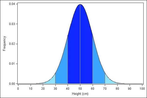
Normal Probability Density Function代写 (a) the Normal Probability Density Function with .Let , then plot with x and y, the result is shown in Fig1-1.

(a) the Normal Probability Density Function with .

Let , then plot with x and y, the result is shown in Fig1-1. This function is also called standard normal distribution.

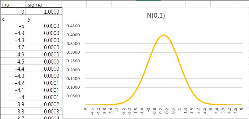
Fig1-1 pdf of normal distribution with

 

(b) graph a normal distribution with , where the result is shown in Fig1-2.

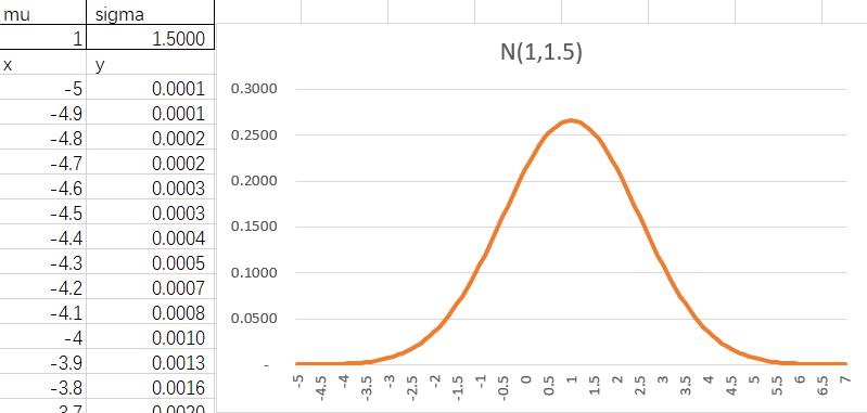
Fig1-2 pdf of normal distribution with

 

(c) Let , x is same as in part(a). Normal Probability Density Function代写

then plot t and y ()

the result is shown in Fig1-3.

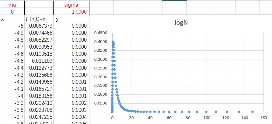
Fig1-3 pdf of log-normal

 

(d) plot another log-normal distribution. the result is shown in Fig1-4.

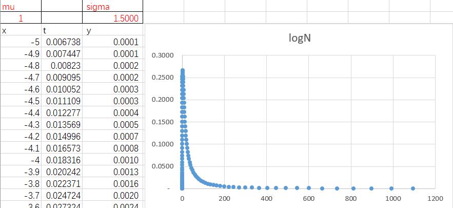
Fig1-4 pdf of log-normal .5

 

Question 2 Normal Probability Density Function代写

(a)

step 1: select the SP200 Index price and Yields on Australian 10-year government bond from 2017-07-06 to 2018-07-06. Data volume of yield on government bond are less than that of SP200 Index. Then, alignment time axis based on the time axis of the bond at first.

Step 2: graph the levels of the above data.

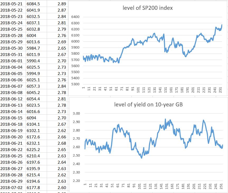
Fig2-1 levels

Step 3: graph the continuous return of SP200 index, . the yield curve of bond is the return curve, which has given in Fig2-1, so, in this step only give the return of SP200 index. The result is shown in Fig2-2.

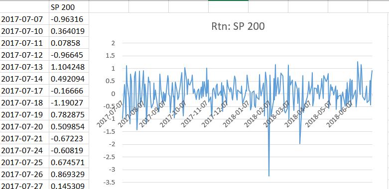
Fig2-2 return

Step 4: scatter plot is shown in Fig2-3.

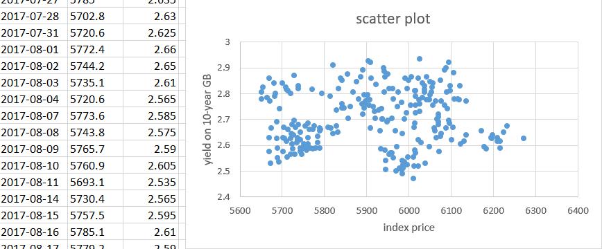
Fig2-3 scatter plot

Step 4: time series plot is shown in Fig2-4.

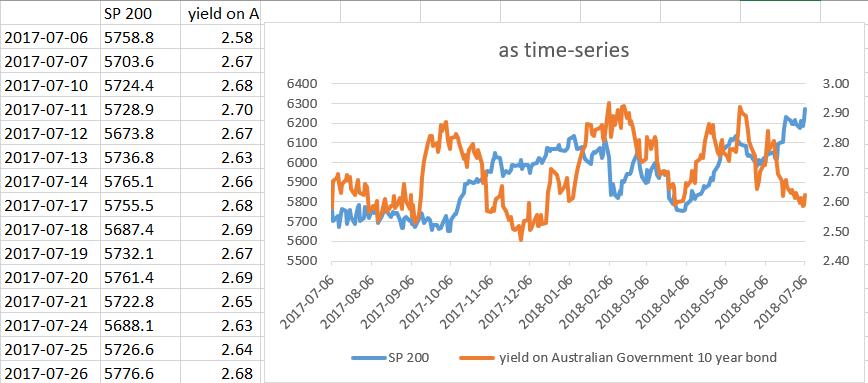
Fig2-4 time-series plot

Step 5: it looks like that SP200 and Government bond are independent. As shown in Fig2-4, when SP200 went up, sometimes yield on Government bond went down (2017-10-03~2017-11-06), and sometimes yield on Government bond went up (2018-04-03~2018-04-24). Normal Probability Density Function代写

 

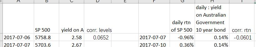
(b) using  function in Excel, we can calculate the correlation coefficient for levels is 0.0652, and the correlation coefficient for returns is -0.0601.

The result shows that the correlation coefficients between MKT and RATE are nearly zero. During a relative long time more than one month, when the MKT reaches a local peak, the RATE may go up. But it still happened both stock market and bond market are bullish.

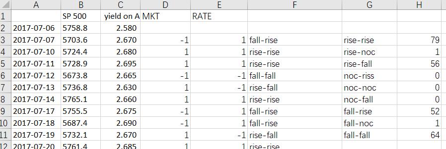
(c) use  function in Excel to count the corresponding numbers.

MKT RATE
		Rise	No change	Fall	Total
	Rise	79	0	52	131
	No change	1	0	1	2
	Fall	56	0	64	120
	Total	136	0	117	253

 

(d) Calculate the joint probability distribution and the marginal probability distributions for the data.

Joint probability distribution: Normal Probability Density Function代写

P {MKT=’Rise’, RATE=’Rise’} = 79/253;

P {MKT=’Rise’, RATE=’No change’} = 1/253;

P {MKT=’Rise’, RATE=’Fall’} = 56/253;

P {MKT=’No change’, RATE=’Rise’} = 0/253=0;

P {MKT=’No change’, RATE=’No change’} = 0/253=0;

P {MKT=’No change’, RATE=’Fall’} = 0/253=0;

P {MKT=’Fall’, RATE=’Rise’} = 52/253;

P {MKT=’Fall’, RATE=’No change’} = 1/253;

P {MKT=’Fall’, RATE=’Fall’} = 64/253;

 

Marginal probability distribution:

P {MKT=’Rise’} = 136/253;

P {MKT=’No change’} = 0/253=0;

P {MKT=’Fall’} = 117/253;

P {RATE=’Rise’} = 131/253;

P {RATE=’No change’} = 2/253;

P {RATE=’Fall’} = 120/253;

 

(e) as P {MKT=’Rise’, RATE=’Rise’} + P {MKT=’No change’, RATE=’No change’}+ P {MKT=’Fall’, RATE=’Fall’} =143/253 > 1/2.

RATE and MKT are weekly positive dependent with each other.

 

(f) conditional probability distribution:

P {MKT=’Rise’| RATE=’Rise’}

= P {MKT=’Rise’, RATE=’Rise’}/ P {RATE=’Rise’} =79/131;

P {MKT=’No change’| RATE=’Rise’}

= P {MKT=’No change’, RATE=’Rise’}/ P {RATE=’Rise’} =0;

P {MKT=’Fall’| RATE=’Rise’}

= P {MKT=’Fall’, RATE=’Rise’}/ P {RATE=’Rise’} =52/131.

 

Question 3 Normal Probability Density Function代写

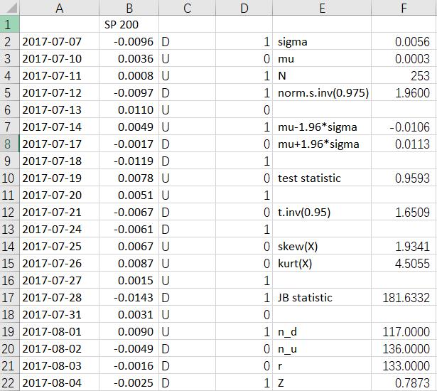
(a) the standard deviation of daily return of SP200 is 0.0055.

The 95 % confidence interval for the daily returns for MKT is

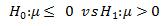
(b) hypothesis test:

testing statistic:

Level of Significance: a = 0.05

Decision rule:

Computation: 

Conclusion: so, we would not reject  at significance level .

they would not invest further in Australian share market using this rule.

(c) hypothesis test:

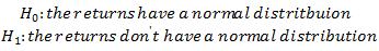
testing statistic:

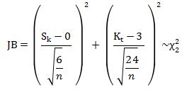
Level of Significance: a = 0.05

Decision rule:

Computation: JB=181.63 > 5.99

Conclusion: so, we would reject  at significance level .

 

As in part(a), we suppose that the daily return is normally distributed, so the result is not accurate, but with large number theory, we also can conclude that the result shown in part(a) is approximately true.

As in part (b), we take student t-distribution as the testing statistic’s approximated distribution, so there is no problem with the result.

(d) runs test

Hypothesis test: 2-tail test

testing statistic:

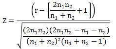
Level of Significance: a = 0.05

Decision rule:

Conclusion: so, we accept  at significance level . That rises and falls are independent.

 

Question 4

(a) at first calculate the simple daily return of SP200 index , and the corresponding daily return of bond .

use Excel add-ins data analysis- regression to conduct this process.

SUMMARY OUTPUT
regression summary
Multiple R	0.02725
R Square	0.00074
Adjusted R Square	-0.00324
stdev	0.00553
number of observations	253
ANOVA
	df	SS	MS	F	Significance F
regression	1	0.0000	0.0000	0.1865	0.6662
residual	251	0.0077	0.0000
Total	252	0.0077
	Coefficients	stdev	t Stat	P-value	Lower 95%	Upper 95%
Intercept	0.0003	0.0003	0.8811	0.3791	-0.0004	0.025725
X Variable 1	-0.0672	0.1556	-0.4318	0.6662	-0.3737	6.235623

 

Also, using Excel function =INTERCEPT(known y’s ,known x’s)

and =SLOPE(known y’s ,known x’s), we can get

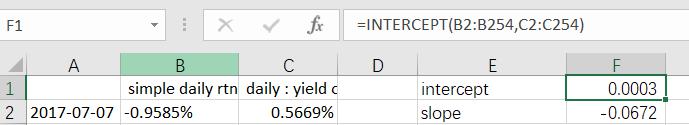
Which is same as using regression method.

As shown in regression summary, e_i² = 0.007868.

The regression equation is MKT_t = 0.0003–0.0672* RATE_{t Normal Probability Density Function代写}

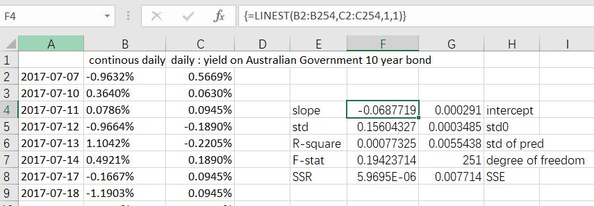
(b) use the continuous return of SP200 index,  then re-estimate the regression equation.

SUMMARY OUTPUT
regression analysis
Multiple R	0.0278
R Square	0.0008
Adjusted R Square	-0.0032
std	0.0055
observations	253
ANOVA
	df	SS	MS	F	Significance F
regression	1	0.0000	0.0000	0.1942	0.6598
residuals	251	0.0077	0.0000
total	252	0.0077
	Coefficients	std	t Stat	P-value	Lower 95%	Upper 95%
Intercept	0.0003	0.0003	0.8350	0.4045	-0.0004	0.0010
X Variable 1	-0.0688	0.1560	-0.4407	0.6598	-0.3761	0.2385

 

The equation is MKT_t = 0.0003–0.0688* RATE_t

 

(c) use excel Function , for both continues MKT return and RATE.

We can get

(d) in part (a) using simple return of Mkt data, in part(b) and part(c) using continuous return of MKT data, there are small difference in coefficients of the equation. But all displays that there are weak negative relationship between return of MKT and return of RATE.

Question 5

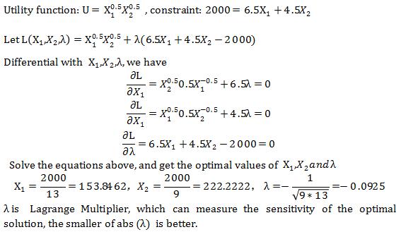
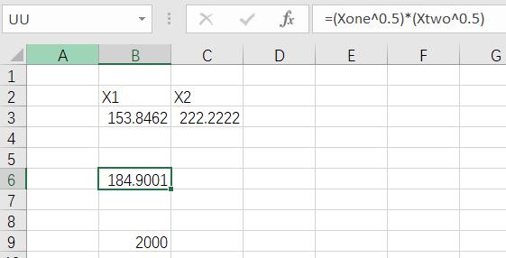
Using Excel solve add-ins we can get the result as below, which is consistent with the result using Lagrange Multiplier Method.

Question 6

(a) dimensions of A, B and C

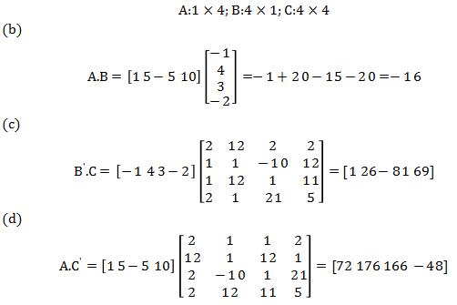
(e) using  function in Excel to compute the matrix product.

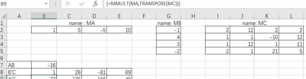
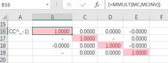
(f) verify that :

Question 7

Step1: calculate the continuous return of each security. Because code: 9305KL and 9217CU has missing values, so take out those two securities. As 2017-12-25, 2017-12-26, 2018-1-1, 2018-1-26, 2018-3-30, 2018-4-2, 2018-4-25,2018-6-11 are Non-trading days, take out the data of those days. then we have 253 days data with 198 tickers.

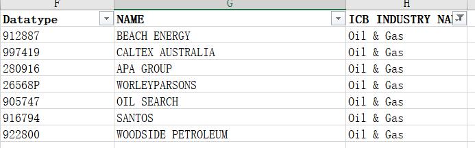
Only those 7 stocks are classified in Oil& Gas.

 

According to the instructions, we can use Excel Solver Tool to find the minimum risk for portfolios for various expected return (about 10 risk-return data)

By changing the values in Twts, we minimum Prsk with constraints :

Wtcn=1, Twts>=0, ret=predefined return of the portfolio.

The result tells that portfolio’s risk is not linear with expected return. When we try expected returns smaller than 0.12, the relative portfolio risk will be increase as the decrease of expected returns; and when we try expected returns larger than 0.12, the relative portfolio risk will increase as the increase of expected returns.

So we should choose the wts that have larger return given the same risk.

 

Question 8 Normal Probability Density Function代写

Step 1: select data of the financial sector components in sheet: Raw Prices for constituents.

And calculate the continuous return, take out non-trading days, and take out the security (9305KL) that has Nas in return.

CODE	BETA	ER	BETASQ	VAR
950706	1.1884	-0.0000	1.4122	0.0065
905209	1.1918	-0.0001	1.4203	0.0066
981800	1.2052	-0.0005	1.4524	0.0098
316588	1.3554	-0.0000	1.8371	0.0102
675493	0.6445	-0.0001	0.4154	0.0135
675667	0.6164	0.0004	0.3800	0.0071
675705	0.9260	0.0007	0.8575	0.0066
691601	0.7410	0.0003	0.5491	0.0105
691992	0.9447	0.0013	0.8924	0.0116
280141	0.5901	0.0006	0.3482	0.0104
314054	1.0925	-0.0004	1.1937	0.0074
502144	0.4248	0.0007	0.1805	0.0081
887937	0.4720	0.0001	0.2228	0.0079
297124	1.0108	0.0007	1.0218	0.0096
263898	1.2014	0.0000	1.4434	0.0148
916763	0.7497	0.0003	0.5620	0.0087
901843	0.9599	0.0007	0.9213	0.0122
26502C	0.7629	0.0009	0.5820	0.0100
503798	0.7578	0.0000	0.5743	0.0088
901842	1.0184	-0.0003	1.0372	0.0064
998066	0.9366	-0.0009	0.8773	0.0126
502192	0.9236	0.0009	0.8531	0.0112
675492	0.7795	-0.0014	0.6077	0.0115
27952T	1.0277	-0.0002	1.0561	0.0129
930388	0.9346	-0.0008	0.8734	0.0108
879286	1.2004	-0.0004	1.4408	0.0135
905506	0.7102	-0.0003	0.5044	0.0092
28516K	1.2524	0.0005	1.5684	0.0120
28836N	1.4916	-0.0007	2.2250	0.0137
754824	0.8594	0.0002	0.7386	0.0093
503969	0.7122	0.0008	0.5072	0.0086
36003D	0.9746	0.0008	0.9498	0.0092
50579C	1.3517	0.0006	1.8270	0.0209
507749	0.5084	0.0006	0.2585	0.0071
865438	1.2219	0.0013	1.4931	0.0087
87867P	0.4081	0.0006	0.1666	0.0078
89592Q	0.9774	0.0002	0.9553	0.0135
8851HK	1.0237	0.0010	1.0479	0.0147
2640K4	0.2664	0.0003	0.0709	0.0083
9105LQ	1.0780	0.0045	1.1622	0.0323
51280P	1.4084	-0.0003	1.9835	0.0146
362569	0.8562	-0.0005	0.7330	0.0132
93650L	0.3855	0.0005	0.1486	0.0096
8866ZY	0.7178	0.0004	0.5152	0.0092
8898YZ	1.0142	-0.0007	1.0286	0.0169
8875U5	0.6669	0.0002	0.4447	0.0108
9387VV	1.2033	-0.0005	1.4480	0.0130
779763	0.5520	0.0001	0.3047	0.0095
95378H	0.5718	0.0007	0.3269	0.0157
27917F	1.2192	-0.0000	1.4863	0.0115
7749ZN	0.4338	-0.0001	0.1882	0.0074

 

Conduct function in Excel to estimate the SML, and we find the slope is -0.0686, and the intercept is 0.1235.

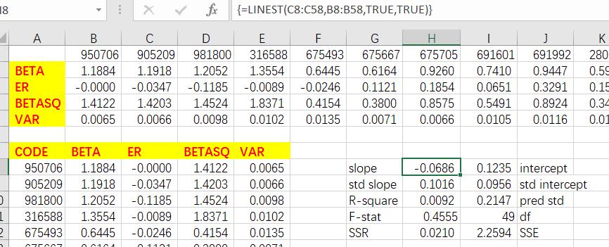
Also, we conduct linear regression using data analysis add-in in excel. Normal Probability Density Function代写

SUMMARY OUTPUT
regression analysis
Multiple R	0.0959703
R Square	0.009210299
Adjusted R Square	-0.011009899
pred std	0.214734946
observations	51
ANOVA
	df	SS	MS	F	Significance F
regression	1	0.021004	0.021004	0.4555	0.502907
residuals	49	2.259444	0.046111
Total	50	2.280447
	Coefficients	std	t Stat	P-value	Lower 95%	Upper 95%
Intercept	0.123518199	0.095569	1.292446	0.202264	-0.06854	0.315572
BETA	-0.068593656	0.101634	-0.67491	0.502907	-0.27284	0.135648

Then, conduct regression process, and we get the following result.

SUMMARY OUTPUT
regression analysis
Multiple R	0.5189451
R Square	0.26930402
Adjusted R Square	0.22266385
pred std	0.18829095
observations	51
ANOVA
	df	SS	MS	F	Significance F
regression	3	0.614134	0.204711	5.774079	0.001906
residuals	47	1.666314	0.035453
Total	50	2.280447
	Coefficients	std	t Stat	P-value	Lower 95%	Upper 95%
Intercept	-0.1589226	0.210921	-0.75347	0.454927	-0.58324	0.265396
BETASQ	-0.1511275	0.277209	-0.54517	0.588211	-0.7088	0.406546
VAR	26.9600738	6.666663	4.044013	0.000194	13.54848	40.37167
BETA	0.06238299	0.49629	0.125699	0.900507	-0.93602	1.060789

 

The coefficient of VAR’s p-value is less than 0.05, which means significant. But the coefficient for BETA and BETASQ is not significant. With more explanatory variables like BETASQ and VAR, the adjusted coefficient of determination (namely adjusted R-square have improved a lot, the latter regression’s adjusted R-square is 0.22>-0.01.

 

t-statistic for BETA is 0.125, for BETASQ is -0.54 and for intercept is -0.75, so the absolute values of these three variables’ t-statistic is less than the critical value t(47, 0.95) =1.68, so BETA, BETASQ, intercept don’t have significant impact on expected returns. As t-statistic for VAR is 4.04>1.68, so, VAR has a significant impact on expected returns.

 

regression function’s coefficients of SML are both insignificant, we doubt that daily returns may have too much noise, maybe monthly returns will perform better. The result in SML regression function shows that the intercept>0,which means the risk-free rate is nearly 0.12, and BETA’s coefficient=-0.06<0, which means the risk-premium of MKT is less than 0.

更多其他:prensentation代写 文学论文代写 商科论文代写 Resume代写 文学论文代写 商科论文代写 艺术论文代写 人文代写

合作平台：天才代写 幽灵代写  写手招聘