Computing Means代写 solution代写 regression代写

Computing Means

Computing Means代写 denote as daily return, as mean of portfolio daily return, as standard deviation of portfolio daily return.

(a) solution:           Computing Means代写

denote  as daily return,  as mean of portfolio daily return,  as standard deviation of portfolio daily return.

clear all; clc

%% import data

data = xlsread(‘Portfolios_Formed_on_Size_Daily.xlsx’,’A4:O22279′);

dt   = data(:,4:15);

meanrtn_daily = 100*mean(dt,1);  % means of returns

stdrtn_daily  = 100*std(dt,0,1);  % std of returns

 

section	CAP1RET	CAP2RET	CAP3RET	CAP4RET	CAP5RET	CAP6RET
	0.0676	0.0537	0.0466	0.0472	0.0454	0.0458
	1.3083	1.1999	1.1343	1.1080	1.1455	1.1323
section	CAP7RET	CAP8RET	CAP9RET	CAP10RET	vwretd	ewretd
	0.0459	0.0419	0.0449	0.0388	0.0401	0.0866
	1.1377	1.1131	1.0937	1.0681	1.0624	1.0604

 

(b) solution:       Computing Means代写

denote  as mean of portfolio monthly return,  as standard deviation of portfolio monthly return. as mean of portfolio annualized return,  as standard deviation of portfolio annualized return. assuming that there are 21 trading days in one month, and 252 trading days in one year, then we have

meanrtn_monthly = 21*meanrtn_daily;

meanrtn_annually= 252*meanrtn_daily;

stdrtn_monthly = sqrt(21)*stdrtn_daily;

stdrtn_annually= sqrt(252)*stdrtn_daily;

 

section	CAP1RET	CAP2RET	CAP3RET	CAP4RET	CAP5RET	CAP6RET
	1.4203	1.1285	0.9792	0.9920	0.9530	0.9608
	5.9952	5.4985	5.1979	5.0774	5.2495	5.1888
section	CAP7RET	CAP8RET	CAP9RET	CAP10RET	vwretd	ewretd
	0.9649	0.8796	0.9434	0.8149	0.8414	1.8182
	5.2137	5.1010	5.0121	4.8945	4.8683	4.8592

 

section	CAP1RET	CAP2RET	CAP3RET	CAP4RET	CAP5RET	CAP6RET
	17.0438	13.5425	11.75	11.9042	11.4358	11.5291
	20.7681	19.0475	18.006	17.5886	18.1849	17.9746
section	CAP7RET	CAP8RET	CAP9RET	CAP10RET	vwretd	ewretd
	11.5792	10.5546	11.3204	9.7784	10.0965	21.818
	18.0607	17.6704	17.3624	16.9549	16.8643	16.8329

 

(c) solution:           Computing Means代写

yes, we can compute the means using a simple regression.

 

With MATLAB command .

We can get the results below, which are equal with the result in part(a).

beta = [];

for i = 1:size(dt,2)

[b,bint,r,rint,stat] = regress(dt(:,i),ones(size(dt,1),1));

beta = [beta,b*100];

end

% check whether beta equals meanrtn_daily

check = round(beta) – round(meanrtn_daily);

 

	CAP1RET	CAP2RET	CAP3RET	CAP4RET	CAP5RET	CAP6RET
beta	0.0676	0.0537	0.0466	0.0472	0.0454	0.0458
	CAP1RET	CAP2RET	CAP3RET	CAP4RET	CAP5RET	CAP6RET
beta	0.0459	0.0419	0.0449	0.0388	0.0401	0.0866

 

(d) solution:

Hypothesis testing:          Computing Means代写

the mean of each portfolios for the pre-1945 and post-1945 subsamples are same.

the mean of each portfolios for the pre-1945 and post-1945 subsamples are different.

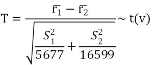
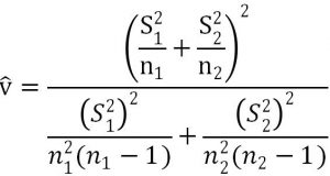
Testing statistic:

Level of Significance: a = 0.1

Decision rule: , reject

Computation: by MATLAB command we can get T =-1.1411, then .

Conclusion: we accept that the mean of each portfolios for the pre-1945 and post-1945 subsamples are same.

presub  =  dt(1:5677,:);     postsub =  dt(5678:end,:);

r_pre = 100*mean(presub,1);  r_post= 100*mean(postsub,1);

n1=size(r_pre,2);  n2=size(r_post,2);

S1 = std(r_pre,0,2);  S2 =std(r_post,0,2);

Sw2 = S1^2/n1+S2^2/n2;

Tstat = (mean(r_pre,2)-mean(r_post,2))/sqrt(Sw2);

v = Sw2^2/(S1^4/n1^2/(n1-1)+S2^4/n2^2/(n2-1));

alpha = 0.05;   % set significance level of 0.05

criticalvalue = tinv(1-alpha/2,v);

if abs(Tstat)>= criticalvalue

disp(‘reject Null Hypothesis’);

else

disp(‘accept Null Hypothesis’);

end

>> accept Null Hypothesis

 

2. Efficient Markets          Computing Means代写

(a) using each of the 11 portfolio returns ( value-weighted and 10 decile portfolio returns), estimate:

Solution:

y = dt(1:end-1,1:11);

x = dt(2:end,1:11);

x0 = ones(size(x,1),1);

clist   = [];

philist = [];

for i = 1:size(y,2)

X = [x0,x(:,i)];

Y = y(:,i);

[b,bint,r,rint,stat] = regress(Y,X);

clist   = [clist,b(1)];

philist = [philist,b(2)];

end

 

(b) test the hypothesis that markets are efficient, i.e. that returns are not serially correlated.

This is known as weak form efficiency (Fama(1970,1990)). Please conduct the test for each portfolio separately.

Solution:

testing = [];

for i = 1:size(y,2)

X = [x0,x(:,i)];

Y = y(:,i);

[b,bint,r,rint,stat] = regress(Y,X);

est_ep=sqrt(stat(4));

C = inv(X’*X);

Tstat = b(2)/(est_ep*sqrt(C(2,2)));

criticalvalue = tinv(1-alpha/2,size(Y,1)-2-1);

 if (abs(Tstat)>= criticalvalue)

disp([num2str(i),‘-th Portfolio: serially correlated, reject Null Hypothesis’]);

temp = 1;

else

disp([num2str(i),‘-th Portfolio: not serially correlated, accept Null Hypothesis’]);

temp = 0;

    end  

testing = [testing;b(2), Tstat, criticalvalue, temp];

end

(c) explain your results.

Solution:

The result runs in part b is

>>1-th Portfolio: serially correlated, reject Null Hypothesis

>>2-th Portfolio: serially correlated, reject Null Hypothesis

>>3-th Portfolio: serially correlated, reject Null Hypothesis

>>4-th Portfolio: serially correlated, reject Null Hypothesis

>>5-th Portfolio: serially correlated, reject Null Hypothesis

>>6-th Portfolio: serially correlated, reject Null Hypothesis

>>7-th Portfolio: serially correlated, reject Null Hypothesis

>>8-th Portfolio: serially correlated, reject Null Hypothesis

>>9-th Portfolio: serially correlated, reject Null Hypothesis

>>10-th Portfolio: serially correlated, reject Null Hypothesis

>>value weighted Portfolio: serially correlated, reject Null Hypothesis

As the testing result shows, all portfolios ‘s return is serially correlated. we can conclude that the market is not efficient enough.

3. Data-Mining

(a) you have no clear model in mind,

but intuition tells you that the returns of small companies might forecast market (value-weighted) returns. therefore, you decide to run the regression:

 

Where  is the return of the value-weighted (market?) portfolio, and  is the lagged return of Decile 1 companies. Run similar regressions for Decile 2 and Decile 3.

Solution:          Computing Means代写

yvw = dt(2:end,11);   % value-weighted returns r_t

x  = dt(1:end-1,1:3);   % decile 1/2/3  r_(t-1)

x0 = ones(size(x,1),1);

datamining = [];

for i = 1:size(x,2)

X = [x0,x(:,i)];

[b,bint,r,rint,stat] = regress(yvw,X);

est_ep=sqrt(stat(4));

C = inv(X’*X);

Tstat = b(2)/(est_ep*sqrt(C(2,2)));

criticalvalue = tinv(1-alpha/2,size(Y,1)-2-1);

 if (abs(Tstat)>= criticalvalue)

disp([num2str(i),‘-th decile Portfolio: significant, can forecast market returns’]);

temp = 1;

   else

disp([num2str(i),‘-th decile Portfolio: not significant, can not forecast market returns’]);

temp = 0;

    end  

datamining = [datamining;b(2), Tstat, criticalvalue, temp];

end

(b) can the return of small companies forecast the market return?

Solution:

The running result in part(a) is:

>>1-th decile Portfolio: significant, can forecast market returns

>>2-th decile Portfolio: significant, can forecast market returns

>>3-th decile Portfolio: significant, can forecast market returns

So, we can conclude that small companies can forecast the market return.

 

4. Simulation:           Computing Means代写

Solution:

%(a) to start the recursion, we need an initial value Y0,let Y0=0

Y0 = 0;

%(b) generate a sequence of Gaussian white noise {epsilon_t} for T=100

T = 100;

Y1= [Y0;NaN(T,1)];

noise = [0;normrnd(0,1,T,1)];

% (c) for phi =0.1, serial 1

phi = 0.1;

for i = 2:T+1

Y1(i) = phi* Y1(i-1)+noise(i);

end

% (d) noise Guassian white noise epsilon

Y2 = [0;NaN(T,1)];

noise2 = [0;normrnd(0,1,T,1)];

% (e) serial 2

for i = 2:T+1

Y2(i) = phi* Y2(i-1)^2+noise2(i);

end

YY = [];

YY = [YY,Y1,Y2];

% (f） repeat b~c

for loop= 3:1000

Y_temp = [Y0;NaN(T,1)];

noise_temp = [0;normrnd(0,1,T,1)];

for i=2:(T+1)

Y_temp(i) = phi*Y_temp(i-1) + noise_temp(i);

    end

YY = [YY,Y_temp];

end

% (g) compute E(Y_t) and Var(Y_t)

% Y_t = e_t + phi* (e_(t_1))+phi^2 * e_(t-2)+…

% EY_t =0

% Var(Y_t) = E(Y^2) = E(e_t+phi*e_(t-1)+phi^2*e_(t-2)+…)

%          = (1+phi^2+phi^4+….)*1

%          = 1/(1-phi^2);

% (h) compute the mean of Y_t across time

muhatN = mean(YY(2:end,:),1);

% (i) compute the mean of Y_t at each t across sectional returns.

muhatT = mean(YY(2:end,:),2);

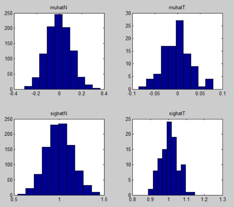
% (j) plot the histogram of the conputed in part h

subplot(2,2,1)

hist(muhatN)

title(‘muhatN’)

% (k) plot the histgram of the computed in part i. Do they vary over time?

subplot(2,2,2)

hist(muhatT)

title(‘muhatT’)

% (l) How do the estimate in h an i compare with the theoretical mean

% E(Y_t) ?

% the simulation values is approximate to 0.

% (m) OPTIONAL: do parts h-k for the second moments.

sighatN = mean(YY(2:end,:).^2,1);

sighatT = mean(YY(2:end,:).^2,2);

subplot(2,2,3)

hist(sighatN)

title(‘sighatN’)

subplot(2,2,4)

hist(sighatT)

title(‘sighatT’)

 

 

更多其他： 数据分析代写  润色修改  代写案例 Essay代写 prensentation代写 Case study代写 Academic代写 Review代写

合作平台：天才代写 幽灵代写  写手招聘