Conservation Law Between Volatility and Fractal Dimension of Currency Exchange Rate
金融市场作业代写 This paper is going to calculate and examine volatility and fractal dimension over ten pairs of time series of currency. The purpose…
Introduction
This paper is going to calculate and examine volatility and fractal dimension over ten pairs of time series of currency. The purpose of evaluating the volatility and fractal dimension is to create the conservation law in building a good sketch about the financial market. As known that the average daily volume is about 575 billion dollars in the Euro-Dollar market which is volatile enough to string changes in the stock market. Stock price is correlated to the change of currency exchanges so it is necessary for investors to gain some knowledge to a predictable range of the price volatility to earn profit or avoid risks.
Assuming rational investors are to be risk-aversion and the stocks are traded in an efficient-market with arbitrage-free prices, any uncertainty about changes of currency prices and interest rates would result in changes in investment decisions and therefore impact the market overall as the volume is huge.
In order to get a comprehensive image of the exchange market, our group used ten actively traded currency pairs with 1000 daily data to construct the model. The currency pairs are the following: EUR/USD, EUR/GBP, EUR/CNY, EUR/JPY, EUR/HKD, USD/CAD, USD/JPY, USD/CNY, USD/HKD, USD/GBP.
In this paper we used the Linear Regression, Ridge Regression and Lasso Regression model to construct the graph and used Dickey-Fuller Tests to test our results. The daily currency prices are defined to be autocorrelated and we are going to test the stationarity. By testing if autocorrelations at all lags are statistically indistinguishable from 0, we can conclude the time series is stationary.
Volatility of Currency Prices 金融市场作业代写
Volatility measures the risk performance of assets such as stocks and currency over a period. It represents the extent to which prices change in relation to the average (Boyte-White, para. 1). In the formulation of investment strategies and portfolio diversification, investors and analysts rely on historical volatility to assess the long-term risk exposures (Boyte-White, para.2). The volatility of prices in the stock market is measured using the standard deviation. High standard deviation is an indication that the prices are highly volatile while low standard deviation values suggest low volatility and risk exposure (Boyte-White, para. 2). Therefore, the volatility measures for the selected currencies provide an ideal system for assessing the risk levels and expected returns.
Volatility also shows the changes in currency prices based on the average prices. When there is a high standard deviation, the individual prices record high movement from the mean unlikely for low deviation. It implies that the prices and expected returns will shift significantly from the average values due to the influence of economic and exchange market conditions (Lahmiri 389).
In the forex market, highly volatile currencies are less preferred due to high chances of losses from exchanges during translations or transactions.
According to portfolio theory, a positive relationship exists between risks and returns. The currencies with high risks are likely to generate more profits for holders unlike the ones with low risk exposures. The risk measures are critical in the determination of expected returns from an investment. The assets with high volatilities tend to yield high returns to investors due to the high risk exposures unlike the ones with low volatilities (Della Corte, Ramadorai and Sarno 25). Investors are sufficiently compensated for assuming high risks in the market. They will review 3the levels of risks for each currency and select appropriate ones based on the risk-return composition. From the selected currencies, there are expectations that there will be varied volatility outcomes given the differences in economic and market exposures.
Fractal Dimension Analysis 金融市场作业代写
The fractal dimension analysis for the selected currency pairs verifies the fractal market hypothesis assumptions. The analysis also tests the presence of fractal properties in the currency time series data. Using the pointwise Holder exponents, the price and return series for the currency pairs will be non-random if there is a steady movement in the prices (Kapecka 17). However, in instances where variances in prices are high, there is an assumption that the prices are random. The relationships between the currencies exhibit binding fractal properties. It also shows low variability of the prices and returns over the three-year period of analysis.
Volatility Computation
def volatility(data):

v = [ ]

for i in range(len(data)):

if len(data)-i >= 100:

v.append(np.std(data[i:i+100])/np.mean(data[i:i+100]))

return v
The python code above is used to compute the Volatility of 100 days of Currency Exchange Rate in a specific time frame, which will return a list of volatilities. The method we implemented to compute for volatility is using a function call, which requires one passing variable. The variable is designed to be the ‘Price’ column of the dataset we downloaded from investing.com, the column should be stored as in a list data structure.
In the function, a loop is used to iterate through the price data list, using python range and length to set the iterate variable as the index of the list instead of the actual value of the list. Within the for loop, a condition check is implemented to check whether there is enough data (100 float numbers) to process the later calculation. Also, The NumPy package is imported for math calculation.
The calculation is straight forward, using the NumPy std function to find the standard deviation of 100 numbers, and using the Numpy mean function to find the average of the 100 numbers, the final step of the calculation would be using standard deviation divide the average to get the volatility. Eventually, store the volatility of each one hundred days into a list and return the volatility list.
Fractal Dimension Computation 金融市场作业代写
def Fractal_Dimension_first_attempt(data):

fd_list = [ ]

for i in range(len(data)):

if len(data) - i >= 100:

data_2 = price_data[i:i+100]

lag1, lag2 = 2, 20

lags = range(lag1, lag2)

tau = [sqrt(std(subtract(data_2[lag:], data_2[:-lag]))) for lag in lags]

m = polyfit(log(lags), log(tau), 1)

if m[0] < 0 and m[1]<0:

m[0] = 0

elif m[0] < 0 and m[1]>0:

m[0] = m[1]

hurst = m[0] * 2

fractal_d = 2 - hurst[0]

fd_list.append(fractal_d)

return fd_list
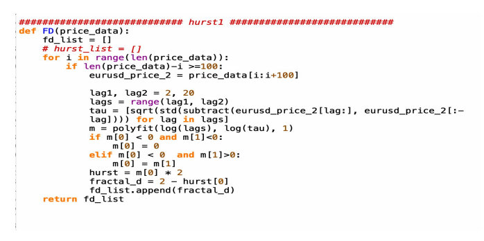
The python code above is the first attempt to get the Fractal Dimension for 100 days of Currency Exchange Rate in a specific time frame. The idea of this code is from Marco Tavora, a physicist and data scientist. This method uses lags as range, computes the tau value using lag function, polyfit the lags and tau to get m value and get the hurst score, then use 2 subtract the hurst score to calculate the Fractal Dimension. However this attempt does not work very well for the later calculation of conservation law.
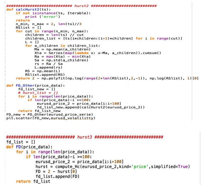
The second attempt we used is provided by Xiaodong Xie, he used R divided by S to get the hurst, we quickly decided to abandon this method, because the process time is very long, also it does not return a very good conservation law result. 金融市场作业代写
def Fractal_Dimension(price_data):

for i in range(len(price_data)):

if len(price_data)-i >=100:

eurusd_price_2 = price_data[i:i+100]

hurst = compute_Hc(eurusd_price_2,kind='price',simplified=True)

FD = 2 - hurst[0]

fd_list.append(FD)

return fd_list
Finally, we decided to get the Fractal Dimension using the compute_Hc function provided by python hurst package (code above), by passing the price list in the function and setting the kind as price and simplified as True, the compute_Hc would return the hurst value. Compared to the first attempt, the process time of the compute_Hc function is shorter, and the Fractal Dimension value fits better with Volatility in the different models for computing the conservation law, resulting in a better R-Square and MSE (mean square error) value.
Linear/Regularization regression
In our project, we used linear and regularization regression to build our prediction model. Linear regression is one of the simplest and most widely used statistical techniques for predictive modeling. In a linear model, the target variable is depending on all independent variables. A general linear regression equation looks like this:

Since in our project, we only have one feature(independent variables). Thus, our linear equation would be: A*Vol(X) + B*FD(Y) = C(a constant). We set C equal to 1 and the goal is to find the coefficients A and B. The coefficients( weights) represent the importance of each independent variable.
If we rewrite our equation based on the general linear regression equation, it will become:

which is our first model, a simple linear regression equation,representing a straight line. Theta 0 is the intercept, and theta1 is the slope of the line.
In our project, we also built the Regularization regression models to compare with the linear regression. Regularization is a process of adding additional information in the model to improve the prediction or to prevent overfitting. One most common way of regularization is adding a constraint to the loss function. Ridge Regression, Lasso are two of the most popular ones.
Ridge regression is also called L2 regularization. It adds a constraint to the model, which is a linear function of the squared coefficients. The general equation of Ridge regression is:

λ is the penalty term, it is the parameter that shows we want to penalize the flexibility of our model to what degree.
Lasso (Least Absolute Shrinkage Selector Operator), known as L1 regularization. It penalizes the model by the absolute value of the weight coefficients.
Lasso’s penalty term is different from ridge regression. It only penalizes the high coefficients by forcing the sum of the absolute value of the coefficients to be less than a constant, thus, some of the coefficients turn to be zero and results in a simpler model.
Our Logic behind the assumption
We will demonstrate our logic behind the assumption step by step. Firstly, let us look at the equation, Y = aX + b. In this equation, Y, the predicted value, will equal to the multiplication of the coefficient and current value of x, plus the intercept. With this formula, we assume that X is the Fractal Dimension and Y is the Volatility. And then, with Linear Regression, we found out the Linear Coefficient and the Intercept. After calculating these values, we got the mean square error and then plotted it. 金融市场作业代写
Let us move to the linear equation, c =aV + bFD, in which c is a constant, a and b are coefficients, V represents Volatility and FD represents Fractal Dimension. This equation is similar to a linear equation; c = aX + bY. Therefore, we can rewrite it as aX + bY – c = 0. For example, it can be something like aX – c = -bY.
Then, we rewrite the value of Y in the following manner: Y = (aX – c) / -b. We can also write it in intercept form: Y = -(a/b) X + c/b.
We assume Fractal Dimension(fd) as the variable on X axis and Volatility (v) as the variable on the Y axis. Since we already know that H = 2 – D, we can use F(fd) instead of D without loss of generality. Now, the value of F lies between 0 and 1. Therefore, the sum of Volatility and Hurst falls between 0 and 2 with an average of 1. This is the reason we assume the constant as 1. Now that we have assumed c = 1, the goal is to find the coefficients a and b.
Therefore we get our equation as: Y = -(a/b) X + 1/b. The value of b is 1/model.intercept and value of a is -1*b*model.coefficient.
Data, Graphs and Accuracy Between Models 金融市场作业代写
In our project, we used three different ways to create conservation law: Linear Regression, Ridge Regression, and Lasso Regression. By comparing these three models, we picked the one who has the largest R-squared and the smallest MSE as our best final model.
The first method is the Linear Regression. To construct the conservation law, we used ten different time series currency pairs, starting from June 12, 2017, to Mar 8, 2020, about three

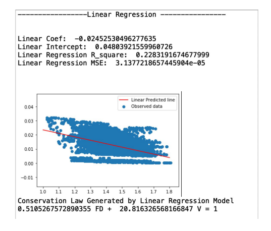
years long, to construct the dataset. We used python to compute FD and V for all ten currency pairs. The scatter plot is shown above, where the x-axis is FD, and the y-axis is V.
After getting FD and V in python, we are able to build the linear relationship for our variables by assuming the constant equals to 1. The Conservation Law generated by Linear Regression Model is 0.5105267572890355 FD + 20.816326568166847 V = 1. In this linear regression model, the result shows that the R-square is 0.22832, which means FD can explain about 22.832% of the Volatility. Meanwhile, the MSE is about 3.1377.
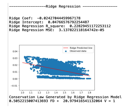
The second alternative method is to use the Ridge Regression model. The result is shown below. The Conservation Law Generated by Ridge Regression Model is 0.5052215007413693 FD + 20.979416541132064 V = 1. We have an R-square equal to 0.22830, and the MSE=3.1378. In this case, we can see the R-square for Ridge Regression is smaller than that of Linear Regression. MSE generated by Ridge Regression is also bigger than the MSE generated by Linear Regression. Therefore, it is clear that after comparing these two models, we can see our conservation law generated by the Linear Regression model is better than the Ridge Regression model.

In order to search a model that better than the above 2. Our group also tested the law by using Lasso Regression. In this case, we have:
Lasso Coef: -0.0
Lasso Intercept: 0.012102210503849496
Lasso Regression R_square: 0.0
Lasso Regression MSE: 4.066087601850162e-05
Our Lasso Regression model yields the highest MSE among the three models. Besides, an 0 value of R-square indicates that V and FD have no relationship, which is not quite true. Therefore, this model is the least accurate one. 金融市场作业代写
Instead of using different models to generate the most accurate conservation law for our project, we also tried three different ways to calculate FD. We found out that each of the methods gave us different processing speed of the system and changed the accuracy of the three models.
After comparing the result of R-Square and MSE from each of the three models, we found out that, by applying Hurst 3 to calculate FD, the speed of processing time has been increased dramatically. The accuracy of R has improved, and MSE has decreased for Linear Regression and Ridge Regression models. Regarding Lasso Regression, even though we changed the way to calculate FD, it didn’t have much influence on the result of this model. The R-Square remains 0, and MSE remains the highest. Hence, Hurst 3 has been applied to our system, and Linear Regression generates the most accurate model for our conservation law. 金融市场作业代写


Conclusion 金融市场作业代写
By testing the above three models, we can conclude that the Linear Regression Model is the most accurate one with smallest MSE value (3.1377) and highest R-square (0.22832) which showed that our data can be 22.832% explained and the mean sum of deviations is about 3.1377 units.
As a conclusion from our findings regarding the financial market, Analysis of Variance (ANOVA), which quantifies the strength of the relationships between variables, is helpful to analyze and evaluate the market performance. According to our tests, Linear Regression is the 12most efficient way of creating the conservation law and also Linear Regression is simple to use compared to others. We can predict the dependent value by the regression model based on changes of independent variable.
In the regression analysis, heteroskedasticity created significant problems for statistical inference. Assuming the volatility of currency pairs presented to be autocorrelated and the estimation of Autoregressive Model for detecting serial correlation is based on linear regression model so testing unit root is a way to test for non-stationarity since a random walk is not covariance stationary. Therefore, testing of AR Model can determine if a time series is covariance stationary and Dicky-Fuller testing should be used.


