STA 137—Applied Time Series Analysis Solutions to Practice Problems I
Time Series代写 1.Let ∇ be the difference operator and specify the quadratic “trend” mt = b0 + b2t2 for some constants b0 and b2. What is ∇2mt?
1.Let ∇ be the difference operator and specify the quadratic “trend” mt = b0 + b2t2 for some constants b0 and b2. What is ∇2mt? [Note: ∇mt = mt − mt−1] Time Series代写
(a)0 (b)b0 (c) 2b2t − b2 (d) 2b2 (e) none of the above
Note that Time Series代写
∇mt = mt − mt−1
= b0 + b2t2 − (b0 + b2[t − 1])2
= b2t2 − b2[t2 − 2t + 1]
= 2b2t − b2
2. Show that the one-sided moving average filter gives exponentially decaying weights to past observations.
Let xt, t ∈ {1, · · · , n} be a time serise and yt is the one-sided moving average
yt = axt + (1 − a)yt−1,
where a ∈ (0, 1) and t ∈ {2, · · · , n}. Hence, Time Series代写
yt = axt + (1 − a)yt−1
= axt + (1 − a){axt−1 + (1 − a)yt−2}
= axt + a(1 − a)xt−1 + (1 − a)2yt−2
.
= axt + a(1 − a)xt−1 + a(1 − a)2xt−2 + · · · + a(1 − a)jxt−j + (1 − a)j+1yt−j−1
It can be seen that the past observation xt−j will be weighted with the factor a(1 − a)j. Since 0 < a < 1, this factor decreases exponentially fast.
3. Let (Yt : t ∈ Z) be a weakly stationary process with mean Define the process (Xt : t ∈ Z) by letting Time Series代写
Xt = st + Yt, t ∈ Z,
where (st : t ∈ Z) is a seasonal component of period d. Apply ∇d to the process (Xt : t ∈ Z) and compute Cov(∇dXt+1, ∇dXt).
The operator ∇d is defined by ∇dXt = Xt − Xt−d. Therefore
Cov(∇dXt+h, ∇dXt) = Cov(Yt+h − Yt+h−d, Yt − Yt−d)
= Cov(Yt+h, Yt) − Cov(Yt+h, Yt−d) − Cov(Yt+h−d, Yt) + Cov(Yt+h−d, Yt−d)
= 2γY (h) − γY (h + d) − γY (h − d),
where γY denotes the ACVF of the weakly stationary process (Yt : t ∈ Z).
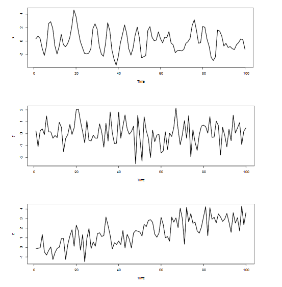
4. In Figure 1, n = 100 observations simulated from time series (Xt), (Yt) and (Zt) are Which of the three processes is not stationary?
(a) (Xt) (b)(Yt) (c) (Zt) (d) none of the processes is stationary
Note that the process in (c) shows an upward trend.

Figure 1: Realizations of (Xt) (top), (Yt) (middle) and (Zt) (bottom).
5. Let(Zt : t ∈ Z) ∼ WN(0, σ2) and let (Xt : t ∈ Z) be given by the equations Time Series代写
Xt = Zt − Zt−1, t ∈ Z.
What are the values of the ACF ρ(h) = Corr(Xt, Xt+h) for h ∈ Z? Compute the ACVF first:
γ(h) = Cov(Xt, Xt+h)
= Cov(Zt − Zt−1, Zt+h − Zt+h−1)
= Cov(Zt, Zt+h) − Cov(Zt, Zt+h−1) − Cov(Zt−1, Zt+h) + Cov(Zt−1, Zt+h−1).
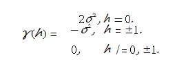
Now the properties of a WN ACVF can be exploited: contributions only appear if the time lags in the two arguments of the covariance function match. This gives

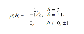
Dividing by γ(0) = 2σ2 gives the ACF values Time Series代写

6.Let(Xt : t ∈ Z) be a stationary process with ACVF γ(h) = exp(−1.5h2) for all h ∈ Z. Give the expression for the ACF ρ(h) at lag h ∈ Z.
Observe that

so that ACVF and ACF coincide.
7. Let(Zt : t ∈ Z) ∼ WN(0, σ2) and let (Xt : t ∈ Z) be given by the equations Time Series代写
Xt = Zt + 0.5Zt−1, t ∈ Z.
Determine ρ(1). (a) 1 (b) 0.5 (c) 0.4 (d) 0
Note that ![]()


